What is imbalanced data?

Let’s dive into the details of these techniques.

These techniques are given by a leading Python Django development company.

List of techniques -:

• Random Undersamopling
• Random Oversampling
• Python imblearn Undersampling
• Python imblearn Oversampling
• Oversampling : SMOTE(Synthetic Minority Oversampling Technique)
• Undersampling: Tomek Links

Looking at imbalanced data

Here, I have collected raw data from here:

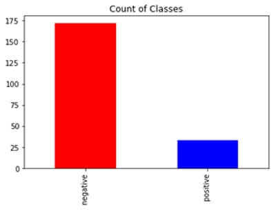
Data is about the classification of glass. It has 2 imbalanced classes, here it is not highly imbalanced but they are imbalanced. Let’s take a look with the help of code.

importpandasaspd importnumpyasnp importmatplotlib.pyplotasplt % matplotlib inline data=pd.read_csv(‘../Data_imb.csv') print(data) Checking the counts of each class data['Class'].value_counts() negative 181 positive 33 Name: Class, dtype: int64 ## Plotting the counts for each class data['Class'].value_counts().plot(kind='bar') <matplotlib.axes._subplots.AxesSubplot at 0x25d838418d0>

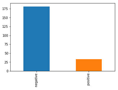
So, here positive class covers about 15% of data which is an imbalance in nature

Now, let’s start looking at techniques to handle this problem.

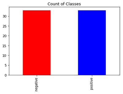
Random Undersampling

In this, what will happen is the majority of class examples will be sampledi.e., some of the examples which belong to the majority class will be removed. It has advantages but, it may cause a lot of information loss in some cases. Let’s look at code, and how to perform undersampling in Python Django development.

count_class_n, count_class_p=data.Class.value_counts() # Divide by class data_class_n=data[data['Class'] ==' negative'] data_class_p=data[data['Class'] ==' positive'] ## Undersampling over negative class(data_class_n) data_class_n_under=data_class_n.sample(count_class_p) ## Concatenating undersamples classes of Negative(undersampled) with the minority class for final data set data_under=pd.concat([data_class_n_under, data_class_p], axis=0) ## Checking the counts of each class after undersampling print('Class count after under-sampling:') print(data_under.Class.value_counts()) ## Plotting the graphs data_under.Class.value_counts().plot(kind='bar', title='Count of Classes') Class count after under-sampling: negative 33 Positive 33 Name: Class, dtype: int64

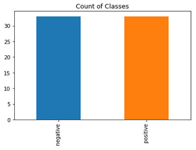
After undersampling, we have 33 data points in each class.

Here undersampling is not a better option because we already have 200 points and after that, we reducing just to 30’s which is less. So, it depends upon the use-case as well.

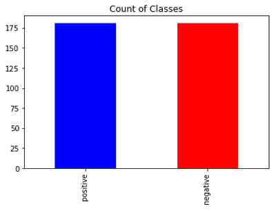
Random Oversampling

Random oversampling will create duplicates of randomly selected examples in the minority class.

## Oversampling over positive class(data_class_p) data_class_p_over=data_class_p.sample(count_class_n, replace=True) ## Concatenating undersamples classes of Positive(Oversampled) with the majority class for final data set data_over=pd.concat([data_class_p_over, data_class_n], axis=0) ## Checking the counts of each class after oversampling print('Class count after under-sampling:') print(data_over.Class.value_counts()) ## Plotting the graphs data_over.Class.value_counts().plot(kind='bar', title='Count of Classes', color=['b','r']) Class count after under-sampling: positive 181 negative 181 Name: Class, dtype: int64 <matplotlib.axes._subplots.AxesSubplot at 0x25d83c85ac8>

Undersampling using Imblearn

Let’s look at undersampling using imblearn package in Python.

Similarly, we can perform oversampling using Imblearn. It might confuse you why to use different libraries for performing undersampling and oversampling. Sometimes, it happens that undersampling(oversampling) using imblearn and simple resampling produces different results and we can select based on the performance as well.

importimblearn fromimblearn.under_samplingimportRandomUnderSampler Undersample=RandomUnderSampler(return_indices=True) ## preparing the data in the format X = data[['RI_real', 'Na_real', 'Mg_real', 'Al_real', 'Si_real', 'K_real', 'Ca_real', 'Ba_real', 'Fe_real']] y =data['Class'] ## Fitting for performing undersampling using imblearn X_rus, y_rus, id_rus=Undersample.fit_sample(X, y) print("Count of class after undersampling") print(pd.Series(y_rus).value_counts()) ## Plotting the graph for class counts after undersampling imblearn pd.Series(y_rus).value_counts().plot(kind='bar', title='Count of Classes', color=['r','b']) Count of class after undersampling negative 33 positive 33 dtype: int64 <matplotlib.axes._subplots.AxesSubplot at 0x25d86471128>

Tomek links

Tomek links is the algorithm based on the distance criteria, instead of removing the data points randomly. It uses distance metrics to remove the points from the majority class. It finds the pair of points that has less distance between them one from the minority class and another from the majority class and will remove the majority point from that pair.

fromimblearn.under_samplingimportTomekLinks ## Creating the Tomeklink object tl=TomekLinks(return_indices=True, ratio='majority') ## Fitting on data X_tl, y_tl, id_tl=tl.fit_sample(X, y) print("Count of class after Tomek-links undersampling") print(pd.Series(y_tl).value_counts()) ## Plotting the class count after the undersampling(Tomeklinks) pd.Series(y_tl).value_counts().plot(kind='bar', title='Count of Classes', color= ['r','b']) Count of class after Tomek-links undersampling negative 172 positive 33 dtype: int64 <matplotlib.axes._subplots.AxesSubplot at 0x25d864360b8>

SMOTE

It stands from the synthetic minority oversampling technique. It also performs oversampling.

fromimblearn.over_samplingimport SMOTE ## Performing the Smote oversampling smote= SMOTE(ratio='minority') X_sm, y_sm=smote.fit_sample(X, y) ## Checking and Plotting the points after smote oversampling print("Count of class after SMOTE undersampling") print(pd.Series(y_sm).value_counts()) pd.Series(y_sm).value_counts().plot(kind='bar', title='Count of Classes', color = ['b','r']) Count of class after undersampling positive 181 negative 181 dtype: int64 <matplotlib.axes._subplots.AxesSubplot at 0x25d863f7eb8>

Conclusion

Hope you are clear with different techniques to overcome with imbalanced dataset in Machine Learning. There are many other methods to deal with imbalance thing. It depends upon your dataset when to perform oversampling and when to perform undersampling. If your dataset is huge then go for undersampling otherwise perform oversampling or TomekLinks.

Hope you enjoyed learning. Keep learning with new stuff in Machine Learning.